Solving Linear Equations
Chapter 2.1, 2.2 Solving Linear Equations.
•As we have seen before, several practical problems lead to
formulation and solution of linear equations. First we see
several examples of this (compare exercises in Chap. 2.1.)
•Production constraints: Suppose we have a 500 acre farm.
Suppose that the production of corn needs $42 per acre while
wheat requires $30 (EX. 2.1.15).
Suppose we have $18, 600 available and we decide to plant in
x acres of corn and y acres of wheat.
What is the mathematical setup of the problem?
•The constraint due to the farm size is:
x + y = 500.
•The constraint due to the available money is:
42x + 30y = 18600.
Samples continued.
•Solving the two equations
x + y = 500 and 42x + 30y = 18600
together gives the answer:
x = 300, y = 200.
•Thus we report the answer: plant 300 acres of corn and
200 acres of wheat!
Investment Example.
•Investment: Two investments yield 8 and 10 percent
annually. If a total of $30, 000 is invested and yield is $2640
per year, how is the fund split between the two investments?
(Compare Chap. 2.1.18)
•We assume that amounts in the two funds (with yields of 8%
and 10% ) are x and y dollars respectively. Then we get the
two constraints:
Net value matched. x + y = 30000
Net return matched. 0.08x + 0.10y = 2640
Answer: Solution gives x = 18, 000 and y = 12, 000.
Diet Example.
•Three kinds of food products give different percentages of
proteins, carbohydrates and iron.
•Name the three products A,B,C. Then we are given:
•Food product A provides 10% of protein, 10% of
carbohydrates and 5% of iron needed daily.
•Food product B provides 6% of protein, 12% of
carbohydrates and 4% of iron needed daily.
•Food product C provides 8% of protein, 6% of carbohydrates
and 12% of iron needed daily.
Calculate how much of each type of food should be eaten to
get the 100% RDA of each food. (Compare Chap. 2.1.25).
•We get three equations:
Protein requirement. 10x + 6y + 8z = 100
Carbohydrate requirement. 10x + 12y + 6z = 100
Iron requirement. 5x + 4y + 12z = 100
•Solution yields:
x = 4, y = 2, z = 6.
•So we recommend that we eat 4 ounces of product A, 2
ounces of product B and 6 ounces of product C.
Real Life Situations.
•Point to note: In real life problems, we shall find that we
don’t get or want exact equations, but rather inequalities.
Also, there is usually some payoff function we are trying to
maximize (or some net cost function we are trying to
minimize).
•This is often accomplished by converting the inequalities to
equations by assigning variable names to the difference
between the two sides of the inequalities.
We will get many possible solutions and develop a method to
optimize our payoff (or cost) function. This is the topic of
Simplex algorithm coming up later.
The plan of action.
•We note that we know everything about how to solve a
system of equations in a single variable.
We also have learnt several techniques to solve two (or more)
equations in two variables.
•For several equations in several variables, the idea is to
extend the old methods to systematically eliminate one
variable at a time and get down to a single variable equation.
•We begin by an example of manipulating equations and then
switch over to a convenient method of manipulating the
matrix of coefficients, thus avoiding the unnecessary
repetition of variable names.
•This is the method of Gauss-Jordan elimination.
Simple Example
•Let us redo the old example of intersecting lines with the new
viewpoint.
Example: Solve
E1 : 3x − y = 5 and E2 : 2x + 3y = 7.
•We shall form the matrix of its coefficients with the variables
mentioned on the top.

•Here RHS stands for the right hand side and the vertical bar
denotes the equality signs.
•We wish to get rid of one of the variables.
•As a good practice, we eliminate the first one in order,
namely x.
•A little thought says that E3 = E2 − (2/3)E1 will give us a new
equation E3 :

•We make a matrix for the new system of E1, E3.

•Clearly we can divide the bottom equation by 11/3 and get
ourselves a new matrix:

Back substitution.
•The current form of our coefficient matrix is said to be in
Row Echelon Form or REF for short.
•It is well suited to solve the last equation for y and then
using that answer, to solve the first for x.
•Typically, we now go back to writing out the current
equations:
3x − y = 5, y = 1.
•Using the y-value from the second equation, we deduce
3x − 1 = 5 or 3x = 6, i.e. x = 2.
This work is called back substitution.
A Bigger Example.
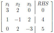
Compare 2.2.4. Start with

•We at once write the coefficient matrix:

•Note that x1 is present in the first equation and the second.
•It is missing from the third.
•We replace the second equation E2 by E2 − (1/3)E1 to get rid of it from E2.
•The new matrix is:

•We have recorded this operation as R2 − (1/3)R1. This means
the second row R2 is replaced by R2 − (1/3)R1.
•Be sure to write the changed row as the first term of the
expression, always!
•The first column is now clean! We work on the second
column next.
The REF.
•Having cleaned x1 column, we also fix the
first row with the
idea that we will use it to solve for x1 at the end.
•In the second column, x2 appears in the second and third
rows. We use the second row entry to clean out the third row
entry.
•The operation used is

•The new matrix is:

Final Answer.
•Our equations are now ready to be solved by back
substitution. The current form of the matrix is said to be
REF (the Row Echelon Form).
•We solve the third equation for x3, namely

•Plug in this value in the second equation and solve for x2.

•Use these values in the first equation to solve:

This gives the final answer:

Conclusion.
•In general, we can follow the same process to solve any
number of equations in many variables.
•In general, our equations will be rearranged such that each
equation has a distinguished variable (called its pivot
variable) which does not appear in lower equations.
•There may be some leftover variables called non pivot
variables.
•Our final answer will express the pivot variables in terms of
the non pivot variables, leaving the non pivot variables free
to take any values! They will be called the free variables.
•Sometimes, we may wipe out all the variables from an
equation. In this case, if the RHS is non zero, then we have
an inconsistent equation and hence no solution. If the whole
equation becomes 0 = 0, then we leave it among the last such
rows. We study this in detail in the next lecture.
|


